HKUST CSIT5401 Recognition System lecture notes 1. 识别系统复习笔记。
- Laplacian Point Detector
- Line Detector
- Edge Detectors
- Scale Invariant Feature Transform (SIFT)
- Harris Corner Detector
Laplacian Point Detector
There are three different types of intensity discontinuities in a digital image:
- Point (Isolated Point)
- Line
- Edge (Ideal, Ramp and Roof)
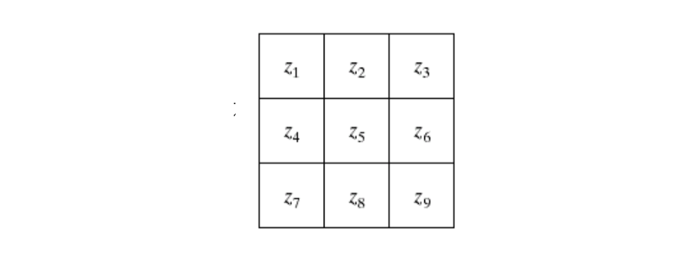
Intensity discountinuity is detected based on the mask response \(R\) within a pre-defined window, e.g. \(3\times3\): \[ R=\sum_{i=1}^9w_iz_i \] where \(w_i\) represent weights within a pre-defined window; \(z_i\) represent intensity values.
If \(|R|≥T\) , then a point has been detected. This point is the location on which the mask is centred, where \(T\) is a non-negative threshold.
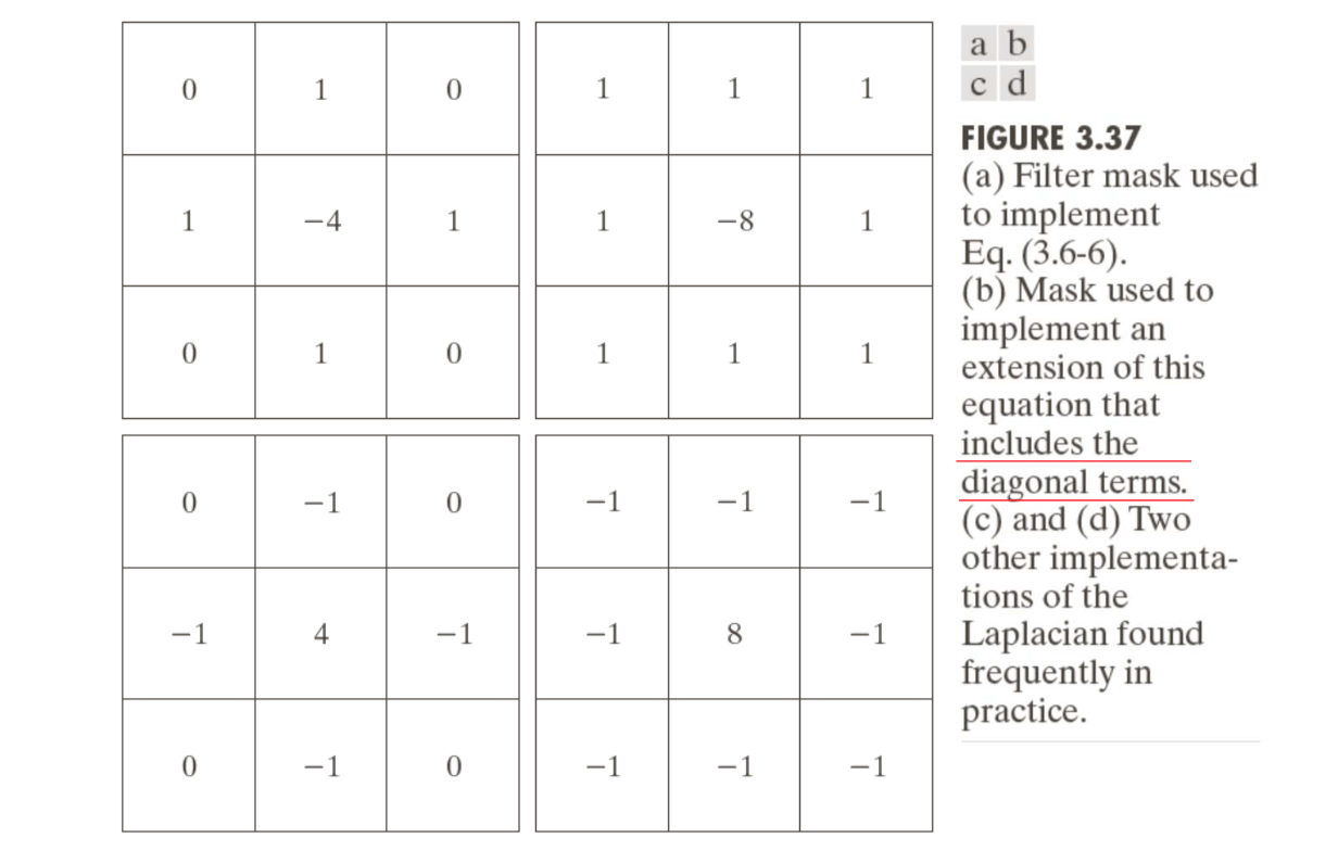
The mask below is the Laplacian mask for detecting point. Sum of all weights is zero to make sure that there is no response at a flat region (constant intensity region).
| 1 | 1 | 1 |
|---|---|---|
| 1 | -8 | 1 |
| 1 | 1 | 1 |
The Laplacian is given as (\(f\) is input image): \[ \triangledown^2f(x,y)=\frac{\partial^2f}{\partial x^2}+\frac{\partial^2 f}{\partial y^2} \] where \[ \frac{\partial^2f}{\partial x^2}=f(x+1,y)-2f(x,y)+f(x-1,y)\\ \frac{\partial^2 f}{\partial y^2}=f(x,y+1)-2f(x,y)+f(x,y-1) \] The discrete implementation of the Laplacian operator is given as: \[ \triangledown^2f(x,y)=f(x+1,y)+f(x-1,y)+f(x,y+1)+f(x,y-1)-4f(x,y) \] Below are several Laplacian masks:
Line Detector
A line is detected when more than one aligned, connected points are detected or, the response of line mask is greater than some threshold. The below are line masks for detecting lines (1 pixel thick) in 4 different specific directions:
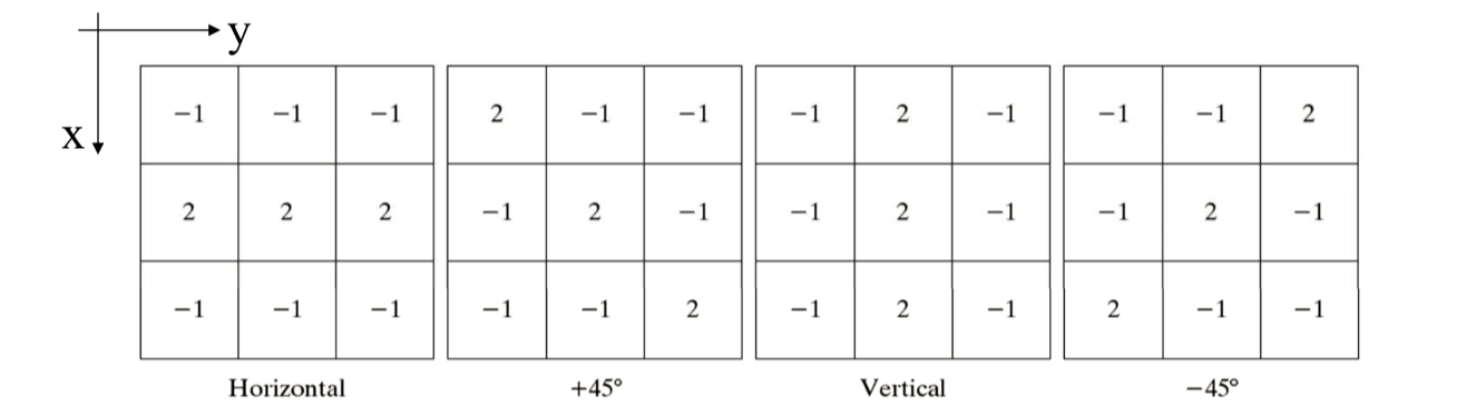
If we want to detect a line in a specified direction, then we should use the mask associated with that direction and threshold its output responses.
If 4 line masks are used, then the final response is equal to the largest response among the masks: \[ R = \max\left(|R_{horizontal}|, |R_{45}|, |R_{vertical}|, |R_{-45}|\right) \] Example code (Matlab):
1 | f = imread('xxx.png'); % read image |
Edge Detectors
Edge is the boundary of regions. The boundary has meaningful discontinuities in grey intensity level. There are three types of edges: ideal edge (left), ramp edge (middle) and roof edge (right).
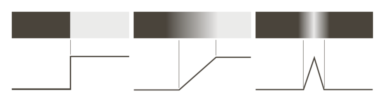
For an ideal edge (step edge, left), an edge is a collection of connected pixels on the region boundary. Ideal edges can occur over the distance of 1 pixel.
Roof edges (right) are models of lines through a region, with the base (width) of a roof edge being determined by the thickness and sharpness of the line. In the limit, when its base is 1 pixel wide, a roof edge becomes a 1 pixel thick line running through a region in an image. Roof edges can represent thin features, e.g., roads, line drawings, etc.
For a ramp edge (middle):
- edge point is any point contained in the ramp
- edge length is determined by the length of the ramp
- the slope of the ramp is inversely proportional to the degree of blurring in the edge
- the first derivative of the intensity profile is positive at the points of transition into and out of the ramp (we move from left to right)
- the second derivative of the intensity profile is positive at the transition associated with the dark side of the edge, and negative at the transition associated with the light side of the edge
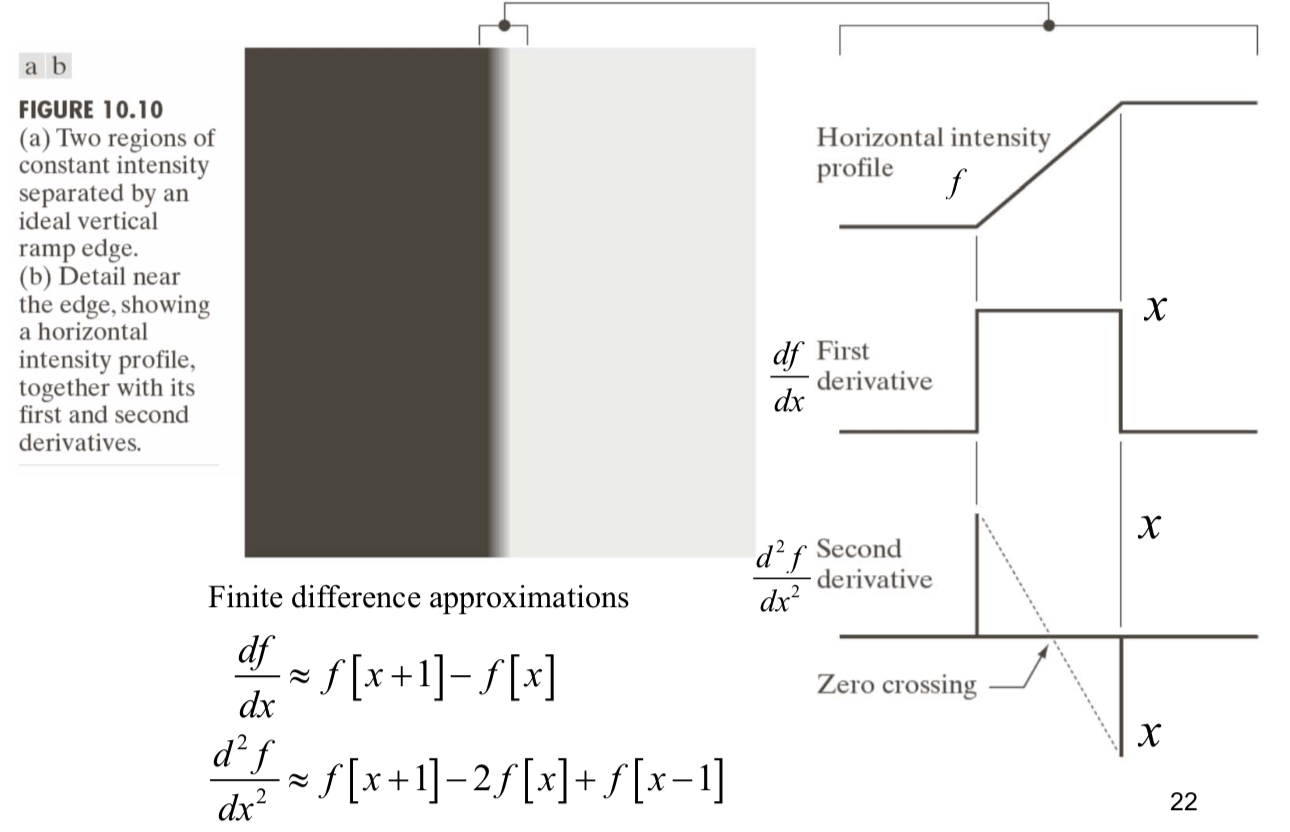
The magnitude of the first derivative can be used to detect the presence of an edge. The sign of the second derivative can be used to determine whether an edge pixel lies on the dark or light side of an edge. The zero-crossing property of the second derivative is very useful for locating the centres of thick edge.
However, fairly little noise can have a significant impact on the first and second derivatives used for edge detection in images. Image smoothing is commonly used prior to the edge detection so that the estimations of the two derivatives can be more accurate.
Gradient Operator
The computation of the gradient of an image is based on obtaining the partial derivatives \(G_x = \partial f/\partial x\) and \(G_y = \partial f/\partial y\) at every pixel location (x,y). The gradient direction and gradient magnitude are \[
\tan^{-1}\left(\frac{G_y}{G_x}\right)\\
|\triangledown f|\approx|G_x|+|G_y|
\] 
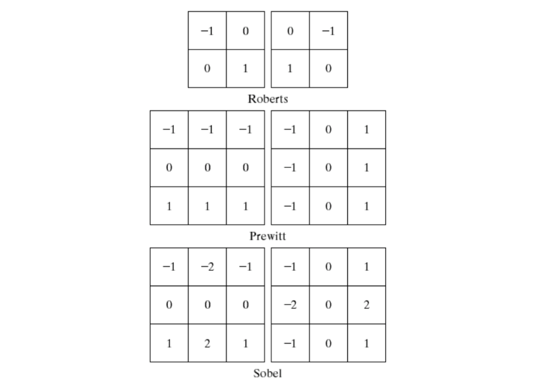
The are several ways to approximate the partial derivatives:
- Roberts cross-gradient operators
- \(G_x = (z_9-z_5)\)
- \(G_y=(z_8-z_6)\)
- Prewitt operators
- \(G_x=(z_7+z_8+z_9)-(z_1+z_2+z_3)\)
- \(G_y=(z_3+z_6+z_9)-(z_1+z_4+z_7)\)
- Sobel operators
- \(G_x=(z_7+2z_8+z_9)-(z_1+2z_2+z_3)\)
- \(G_y=(z_3+2z_6+z_9)-(z_1+2z_4+z_7)\)
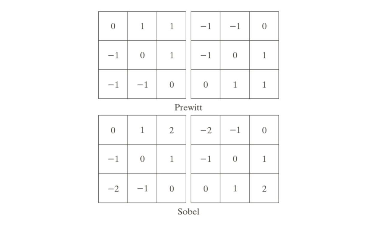
Below are diagonal edge masks for detecting discontinuities in the diagonal directions.
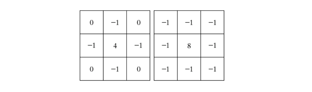
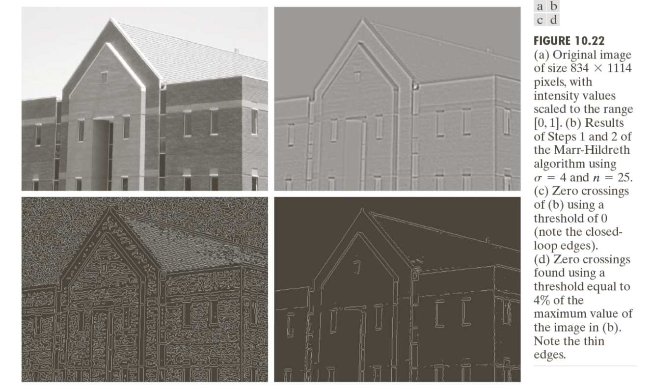
Marr-Hildreth Edge Detector
The Laplacian of an image f(x,y) at location (x,y) is defined as \[ \triangledown^2f(x,y)=\frac{\partial^2f}{\partial x^2}+\frac{\partial^2 f}{\partial y^2} \] There are two approximations: \[ \triangledown^2f=4z_5-(z_2+z_4+z_6+z_8)\\ \triangledown^2f=8z_5-(z_1+z_2+z_3+z_4+z_6+z_7+z_8+z_9) \] The Laplacian generally is not used in its original form for edge detection (based on zero-crossing property) because it is unacceptably sensitive to noise. We smooth the image by using a Gaussian blurring function \(G(r)\), where \(r\) = radius, before we apply the Laplacian operator: \[ G(r)=\exp(\frac{-r^2}{2\sigma^2}) \] The Laplacian of a Gaussian (LoG) operator is defined by \[ \text{LoG}(f)=\triangledown^2(f\ast G)=f\ast(\triangledown^2G) \] Using the LoG, the location of edges can be detected reliably based on the zero-crossing values because image noise level is reduced by the Gaussian function.
Marr-Hildreth algorithm
Filter the input with an n-by-n Gaussian blurring filter \(G(r)\).
Compute the Laplacian of the image resulting from Step 1 using one of the following 3-by-3 masks.
Find the zero crossings of the image from Step 2.
- A zero crossing at a pixel implies that the signs of at least two of its opposing neighboring pixels must be different.
- There are four cases to test: left/right, up/down, and the two diagonals.
- For testing, the signs of the two opposing neighboring pixels must be different and their absolute Laplacian values must be larger than or equal to some threshold.
- If yes, we call the current pixel a zero-crossing pixel.
Scale Invariant Feature Transform (SIFT)
SIFT is useful for finding distinctive patches (keypoints) in images and transforming keypoints (locations) into features vectors for recognition tasks.
SIFT consists of four steps:
- Scale-space extrema detection
- Keypoint localization
- Orientation assignment
- Keypoint descriptor
SIFT feature is
- invariant to image rotation and scale
- partially invariant to change in illumination and 3D camera viewpoint
The method is a cascade (one step followed by the other step) filtering approach, in which more computationally expensive operations are applied only at locations that pass an initial test.
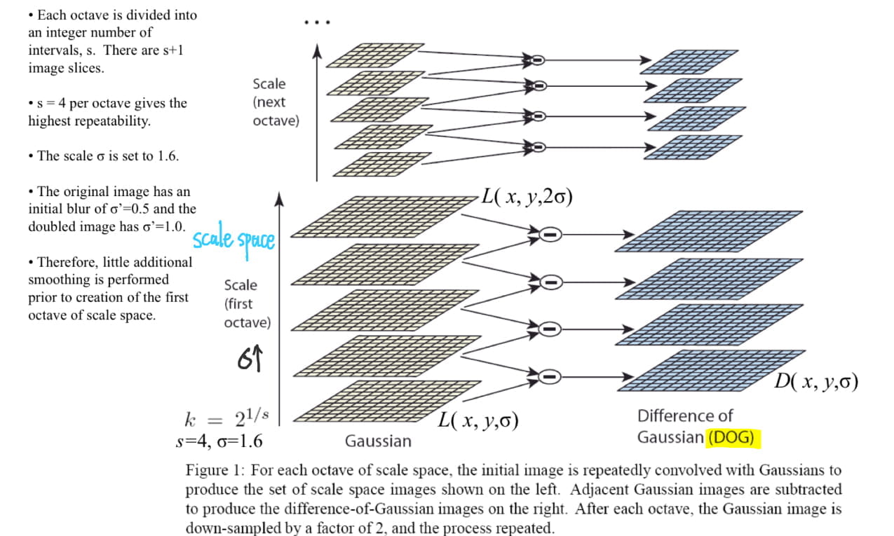
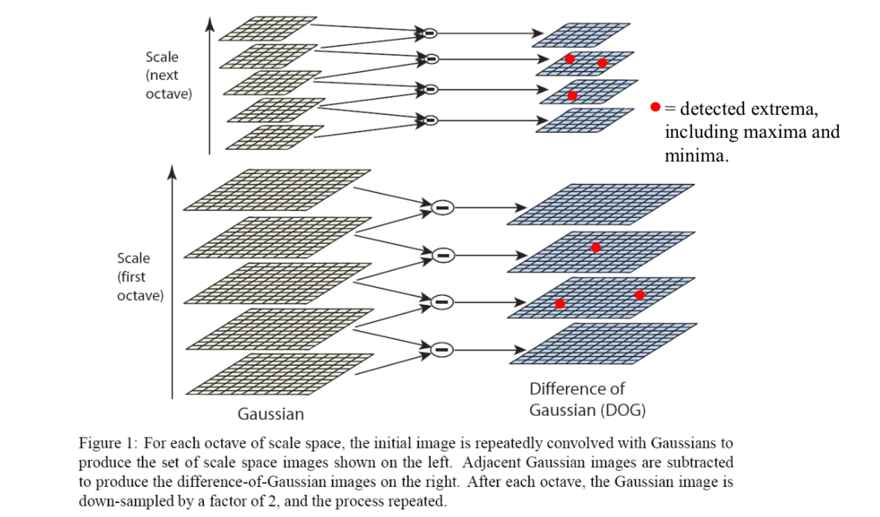
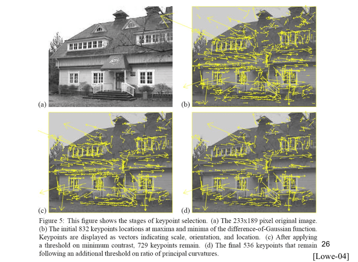
[1] Scale-space extrema detection
Candidate locations are identified by searching for stable features across all scales in the scale space. The scale space of an image is defined as \[ L(x,y,\sigma)=G(x,y,\sigma)\ast I(x,y)\\ G(x,y,\sigma)=\frac{1}{2\pi\sigma^2}\exp(-\frac{x^2+y^2}{2\sigma^2}) \] , where \(\ast\) is the convolution operator (filtering operation), the variable-scale Gaussian is \(G(x, y, \sigma)\) and the image is \(I(s, y)\).
The difference between two nearby scales separated by a constant multiplicative factor \(k\) is \[ \begin{align} D(x,y,\sigma)&=L(x,y,k\sigma)-L(x,y,\sigma)\\ &=\left(G(x,y,k\sigma)-G(x,y,\sigma)\right)\ast I(x,y) \end{align} \] The DoG function provides a close and efficient approximation to the scale-normalized Laplacian of Gaussian (LoG).
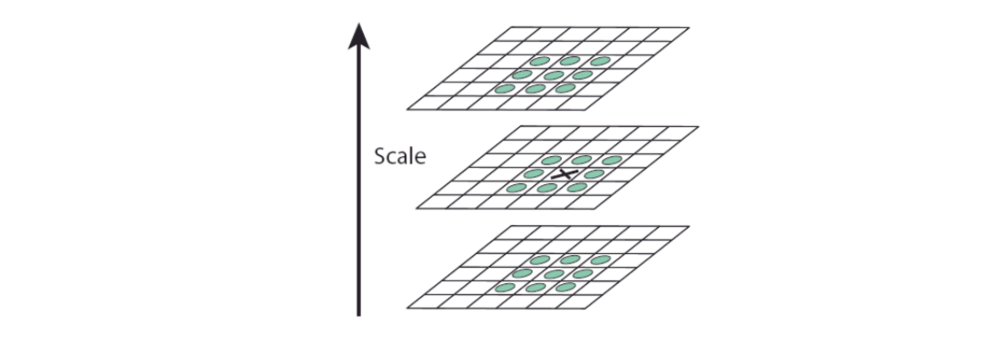
Local extrema (maxima and minima) of \(D( x, y, σ)\) are detected by comparing the values of its 26 neighbors, including 9 from the above image, 9 from bottom image and 8 from the current image.It is selected only if the center pixel is larger than all of these neighbors (26 neighbors) or smaller than all of them.
[2] Keypoint localization
Once a keypoint candidate has been found by comparing a pixel to its neighbors, the next step is to determine whether the keypoint is selected based on local contrast and localization along edge. Therefore, the keypoints will be rejected if these points have low contrast.
All extrema are discarded if \(|D(x)|<0.03\) (minimum contrast), where \(x\) represents a relative image position with maximum value of \(D\). The keypoints will be rejected if these points are poorly localized along an edge (determined based on the ratio of principle curvatures).
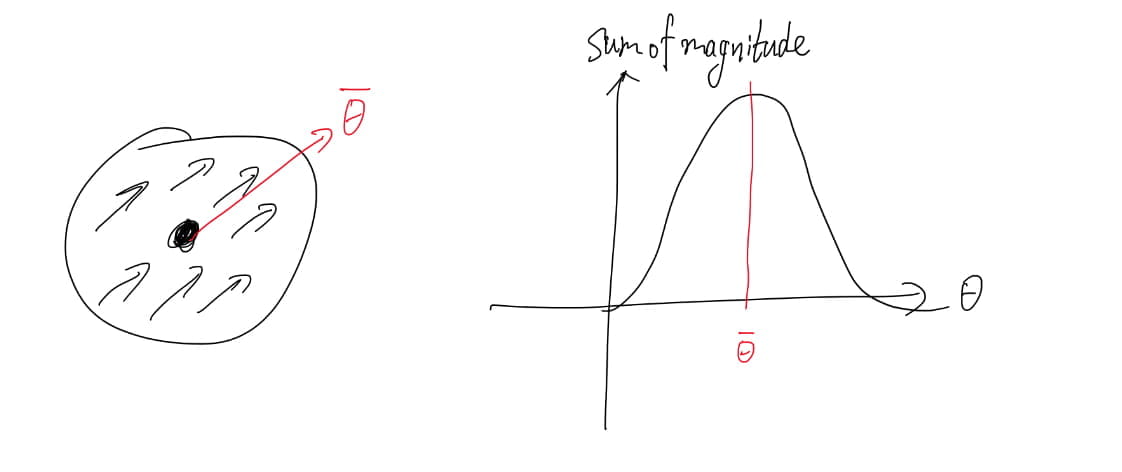
[3] Orientation assignment
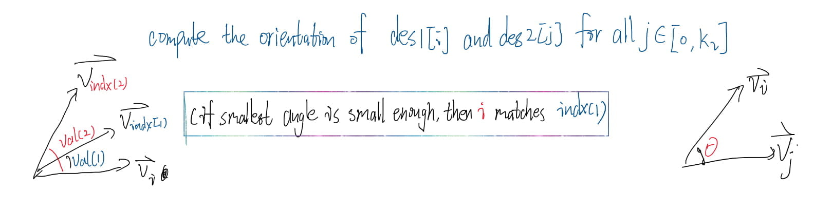
Each corresponding keypoint in \(L\) is assigned a dominant orientation. The keypoint descriptor can be represented relative to this orientation and therefore achieve invariance to image rotation.
The gradient magnitude and orientation are \[ m(x,y)=\sqrt{(L(x+1,y)-L(x-1,y))^2+(L(x,y+1)-L(x,y-1))^2}\\ \theta(x,y)=\tan^{-1}\left(\frac{L(x,y+1)-L(x,y-1)}{L(x+1,y)-L(x-1,y)}\right) \] An orientation histogram is formed from the gradient orientations within a region around the keypoint. The orientation histogram has 36 bins covering the 360 degree range of orientations, 10 degrees per bin. Each sample added to the histogram is weighted by its gradient magnitude and by a Gaussian-weighted circular window (with σ that is 1.5 times that of the scale of the keypoint, and it is related to effective window size). Peak in the orientation histogram corresponds to dominant direction of the local gradients.
[4] Descriptor for local image region
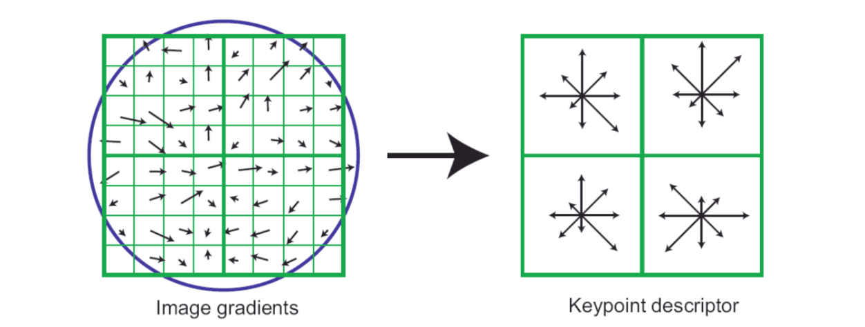
For each detected keypoint, a local image descriptor is computed. It is partially invariant to change in illumination and 3D viewpoint.
In order to achieve orientation invariance, the coordinates and the gradient orientations are rotated relative to the keypoint orientation. A Gaussian weighting function with σ equal to one half the width of the descriptor window is used to assign a weight to the magnitude of each sample point.
Each subregion generates an orientation histogram with 8 orientation bins. Therefore, for each keypoint, if \(2\times2\) descriptor is used, a feature vector can be formed with \(2\times2\times8 = 32\) elements; if \(4\times4\) descriptor is used, there will be \(4\times4\times8 = 128\) elements in a feature vector. The optimal setting is 4x4 subregions and 8 orientation bins (the above picture).
Feature matching
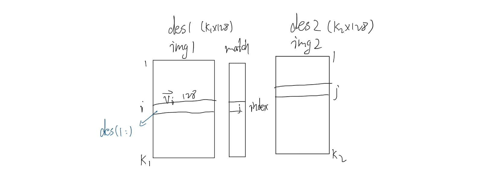
Matlab Implementation
1 | % num = match(image1, image2) |
Harris Corner Detector
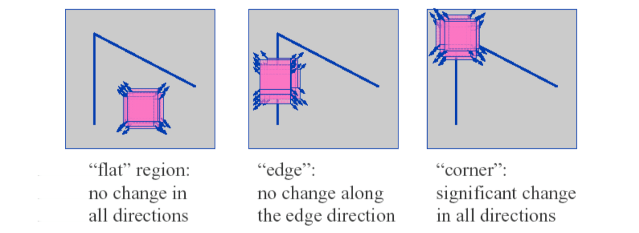
Basic Idea
We should easily recognize the point by looking at intensity values within a small window. hifting the window in any direction should yield a large change in appearance.
Harris corner detector gives a mathematical approach for determining which case holds.
Change of intensity for the shift \([u, v]\): \[ E(u,v)=\sum_{x,y}w(x,y)[I(x+u,y+v)-I(x,y)] \] where \(w(x,y)\) is window function.
For nearly constant patches, this will be near 0. For very distinctive patches, this will be larger. Hence... we want patches where \(E(u,v)\) is LARGE.
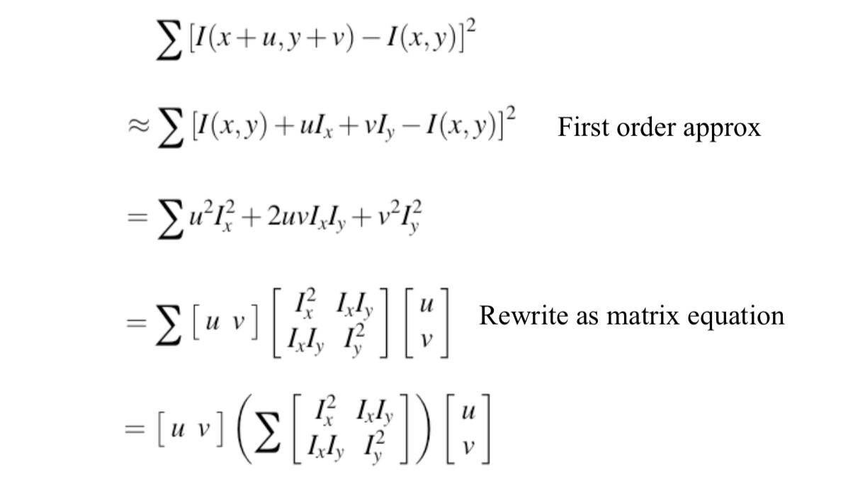
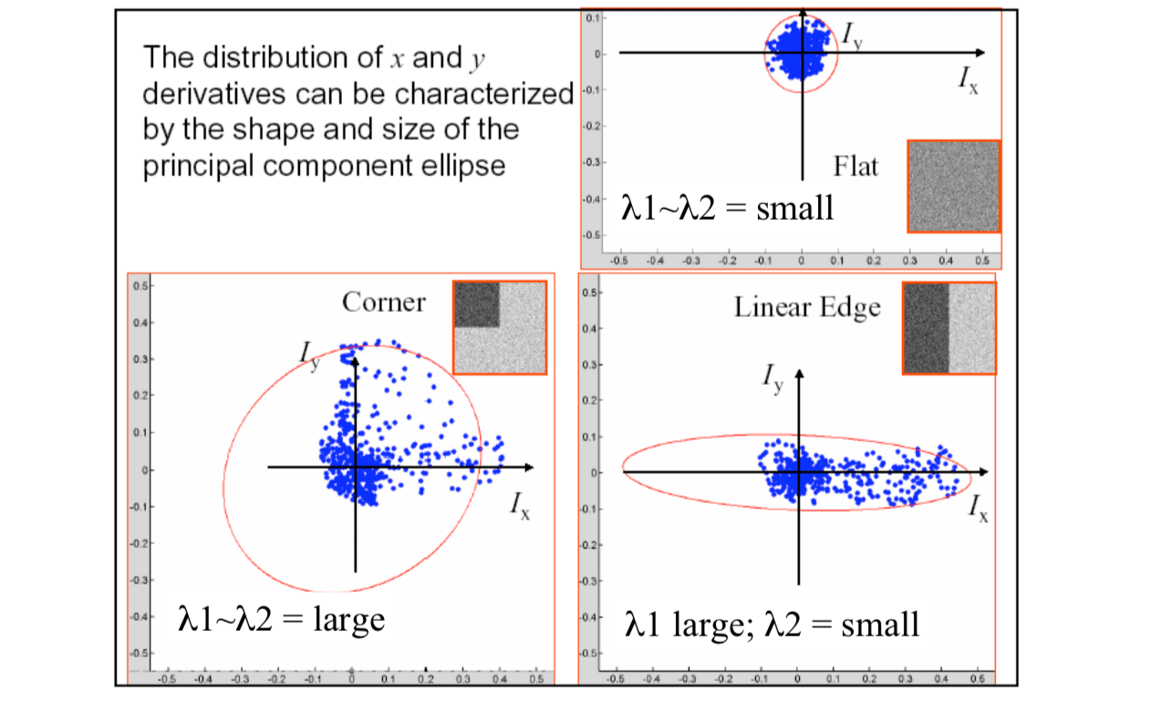
For small shifts \([u, v]\), we have a bilinear approximation: \[ E(u,v)\approx [u,v]M[u,v]^T \] where \(M\) is a 2x2 matrix computed from image derivatives: \[ M=\sum_{x,y}w(x,y)\begin{bmatrix} I_x^2 & I_xI_y \\ I_xI_y & I_y^2 \end{bmatrix} \] Treat gradient vectors as a set of \((dx,dy)\) points with a center of mass defined as being at \((0,0)\). Fit an ellipse to that set of points via scatter matrix.
Measure of corner response: \[ R=Det(M)-k(Trace(M))^2 \] where \[ Det(M)=\lambda_1\lambda_2\\ Trace(M)=\lambda_1+\lambda_2 \] According to \(R\), we can detect corner:
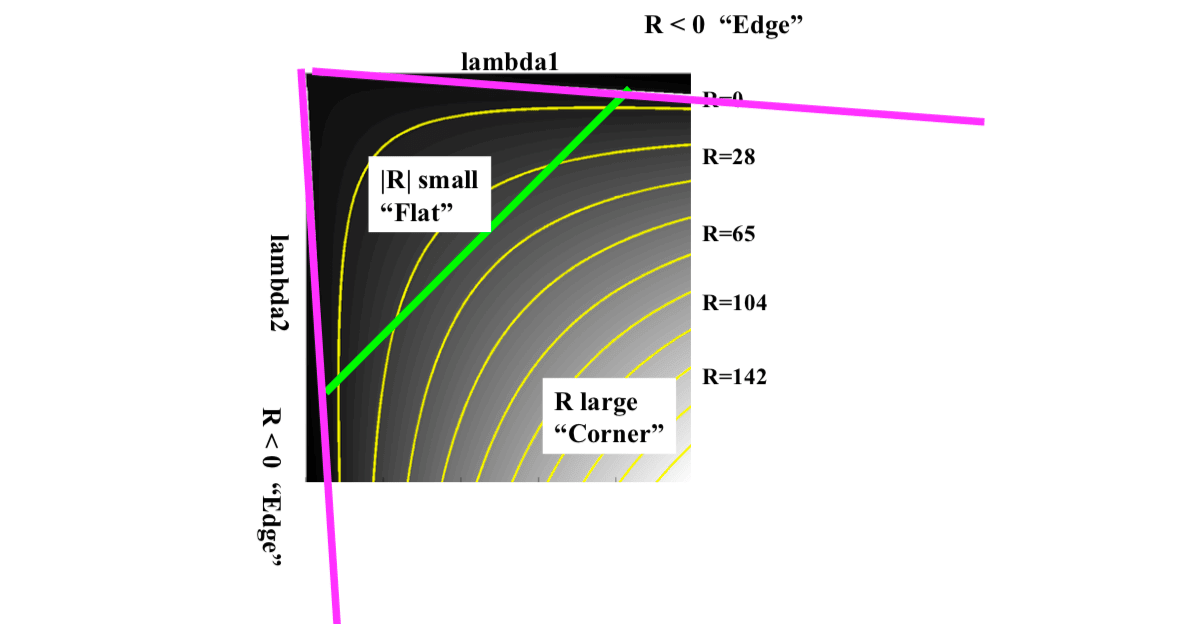
\(R\) depends only on eigenvalues of \(M\). As we can see from figure above,
- \(R\) is large for a corner.
- \(R\) is negative with large magnitude for an edge
- \(|R|\) is small for a flat region
Harris Corner Detection Algorithm
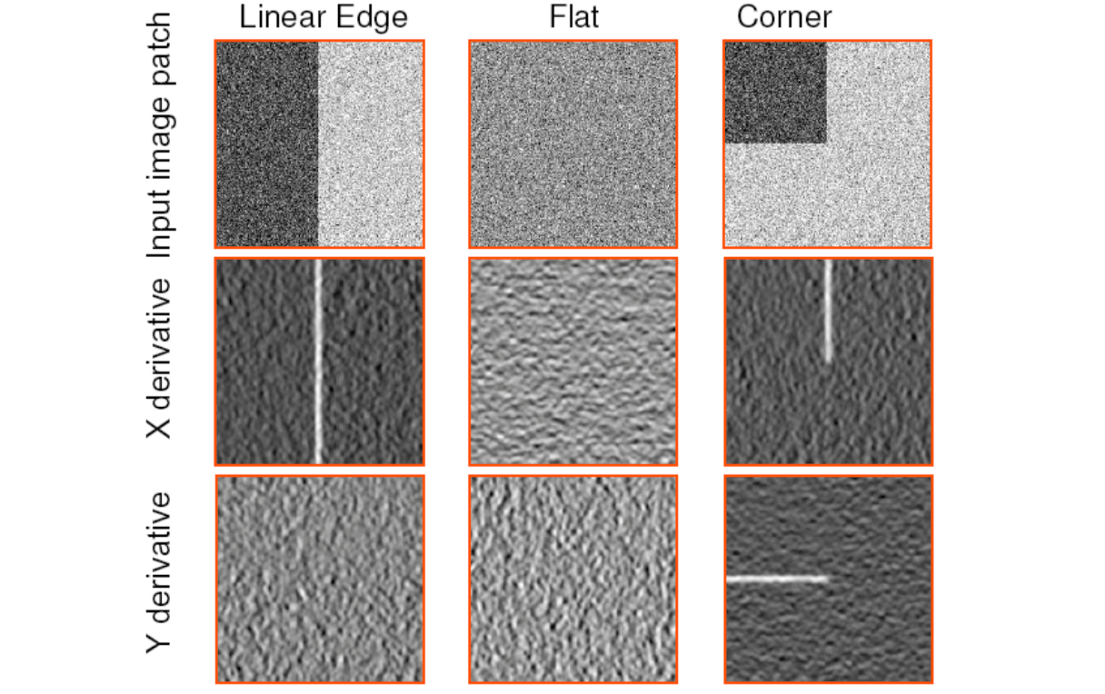
Compute \(x\) and \(y\) derivatives of image: \[ I_x=G_\sigma^x\ast I\\ I_y=G_\sigma^y\ast I \]
Compute products of derivatives at every pixel: \[ I_x^2=I_x\cdot I_x\\ I_y^2=I_y\cdot I_y\\ I_{xy}=I_x\cdot I_y \]
Compute the sums of the products of derrivatives at each pixel: \[ S_x^2=G_\sigma'\ast I_x^2\\ S_y^2=G_\sigma'\ast I_y^2\\ S_{xy}=G_\sigma'\ast I_{xy} \]
Define at each pixel \((x,y)\) the matrix: \[ M(x,y)=\begin{bmatrix} S_x^2(x,y) & S_{xy}(x,y) \\ S_{xy}(x,y) & S_y^2(x,y) \end{bmatrix} \]
Compute the response of the detector at each pixel: \[ R=Det(M)-k(Trace(M))^2 \]
Threshold of value of \(R\). Compute nonmax suppression.